In navigation, when two LOPs (lines of position) are obtained at practically the same time, their intersection is the location of the vessel. But what does a navigator do with non-simultaneous LOPs? A traditional method in this case is to advance the previous LOP to the time of the most recent LOP, just as one would advance the vessel on the chart from its present position to some later time. The intersection of the advanced LOP and second LOP is called a running fix.
A second method is to apply each LOP immediately to the vessel's EP (estimated position: the best estimate of the position, taking into account all factors such as current). The LOP and EP at the time of the LOP are plotted, then the EP is adjusted to the nearest point on the LOP. I.e., the new EP is the point on the LOP that is as close as possible to the old EP. I shall call this an estimated fix to make it explicit that the EP has adjusted to agree with a LOP.
Clearly an estimated fix is simpler to plot than a running fix. But is it equally accurate? To investigate that question I wrote a program to numerically simulate both methods.
The program uses a Monte Carlo method, in which a random number generator simulates navigational errors and causes the LOPs to assume a variety of orientations. To make the problem easier to program, I make some simplifying assumptions:
With those assumptions, the analysis is performed on a Cartesian (rectangular) coordinate system in which the origin is the true position of the vessel. The running fix algorithm is:
The estimated fix algorithm is:
Both algorithms add the same errors in step 1 and use the same LOPs in step 2. That is, I simulate two separate navigators who are provided with identical LOPs and have identical errors when advancing a LOP or EP to a later time.
A running fix is independent of any error in the vessel's position. Only the run of the vessel (i.e., the change in position) from one LOP to the next affects the running fix. On the other hand, because an estimated fix is based on the EP and one LOP, any error in the EP affects the fix. So what EP is used in the running fix algorithm, step 1, when the program starts? We have to begin with something! The answer is that an initial position is obtained by applying the random and systematic errors to an initial perfect position. Then 10 iterations of the fix cycle bring the EP to a reasonable starting state. The statistics from this "warm up" are ignored.
A Windows executable and my C# source code may be downloaded free. To just run the program, only the .exe file is needed. The .cs files are text files of source code in the C# language. They are of interest if you want to see how the program works.
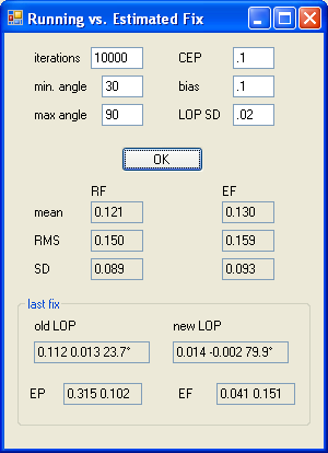
The program is a Windows Forms application, which is simple to write but specifies all visual components in absolute pixels. Therefore, the window cannot be resized by the user. (What do you expect for free?) The screen shot below is actual size.
The Monte Carlo simulation program looks like this:
The white text boxes may be changed by the user. All others display the results from the simulation run.
iterations tells the program how many fixes to perform when OK is clicked. It may be set as low as 1. Each run of the program begins where the last run stopped. That is, the next run begins from the previous LOP and position. Thus, if iterations is 1, you can step through a simulated voyage one fix at a time. (But if any setting is changed, this is not true because the program automatically re-initializes with the new setting, thereby erasing the previous "plot".)
min angle and max angle control the angle between the LOPs. The minimum must be greater than zero. The maximum must be greater than the minimum and not greater than 90, which is the largest possible angle between LOPs. (Because, for example, 100 degrees is the same as 80.) Each new LOP will be oriented at a random direction within the selected range with respect to the previous LOP.
CEP is the circular error probable of the random error applied in step 1 of the algorithm. The probability that this error will be less than the CEP is 50%. The unit of measure is the actual distance traveled by the vessel between LOPs. For example, in the screen shot the CEP is 10% of the distance traveled between LOPs. (Recall that the vessel moves at constant velocity and the LOPs are obtained at equal intervals. Since the distance traveled between LOPs is always the same, it may be used as the unit of distance. This eliminates the requirement to pick a specific speed in knots and a specific elapsed time between LOPs.)
bias is the systematic (constant) error applied in step 1 of the algorithm. It always acts in the +x direction.
LOP SD is the standard deviation of the random Gaussian error applied to each LOP to simulate observation error.
The next part of the screen displays the running fix and estimated fix statistics: the mean error, the square root of the mean squared error, and the standard deviation of the errors.
Finally, at the bottom is a box which shows the geometry of the last fix. This is mainly of interest if the program is run in single step mode (iterations = 1). The data here are sufficient to draw a diagram of both types of fix.
In the old LOP box is the x and y error of the advanced LOP, and its orientation. For example, to draw the advanced LOP in the screen shot example, plot a point at (0.112, 0.013), then draw the LOP through the point at a 23.7° angle. The angle is measured in the usual Cartesian sense: increasing counterclockwise from zero in the +x axis direction. It's always between 0 and 180° because any larger angle can be reduced to an equivalent in that range. Note that the random component of the xy error can be determined because the systematic component is known and always acts in the +x direction. For example, in the screen shot the systematic error ("bias") is 0.1, so the random error was (0.112 - 0.1, 0.013) = (0.012, 0.013).
The new LOP box is similar to old LOP, but generally its x and y are closer to the origin since it does not have the errors that occur when advancing a LOP.
EP is the coordinates (or equivalently, the error) of the EP before it's corrected by the new LOP. It includes the error of the last estimated fix, plus the error of advancing it. The latter is the same as xy error in the old LOP box.
EF is the estimated fix. It displays the coordinates of the point on the new LOP that is as close as possible to the old EP.
With the program defaults (CEP = bias = 0.1, LOP SD = .02, LOP angles = 30 to 90 degrees), the running fix is slightly better than the estimated fix. RMS errors are 0.150 vs. 0.159 respectively. The smaller the angle between LOPs, the more advantage for the running fix. For angles in the range 30 - 40, RMS error is 0.199 vs. 0.310. But for angles in the range 80 - 90, both methods are equal at 0.115.
A pure random error (CEP = 0.1, bias = 0, LOP SD = .02, LOP angles 30 - 90) favors the estimated fix. RMS errors are 0.115 vs. 0.105. Even if LOPs are restricted to the range 30 - 40, both methods are practically equal at 0.156 and 0.154.
On the other hand, a pure systematic error (CEP = 0, bias = 0.1, LOP SD = 0, LOP angles 30 - 90) favors the running fix. RMS errors are 0.092 vs. 0.112. If the LOP angle is restricted to the range 30 - 40, the advantage increases to 0.125 vs. 0.276. In the range 80 - 90 both methods are equal at 0.072.
To summarize, a large systematic error (relative to the random error) favors the running fix, the more so as the angle between LOPs decreases. On the other hand, if the error is entirely random, the estimated fix is more accurate than the running fix when there is a large angle between the LOPs, and equally accurate at small angles.
Those statistics were obtained with runs of 10,000 iterations. The accuracy difference between a running fix and estimated fix depends highly on the fix geometry. This becomes apparent if you select a single iteration per run; it then becomes difficult to make conclusions due to the statistical noise.
[up one level in the site hierarchy]
(page last modified 2013-10-28)